Probability vs Density

30 Dec 2017

Probability is a weird child of math and science. One wants to quantify how uncertain one is with given knowledge. But to top it off is the weirder pet in the family - probability density.

“I mean, what?”

-sizhky

Who wants to know how densely uncertain one is? To talk about density in normal science one needs a normalizing factor. Like how heavy is something per m³. Where is that per-ness in a probability density function?

It doesn’t even make sense.

Until it does. And once I understood it, it was brilliant.

Well, not really. The last sentence was click-bait. Now you feel betrayed. You may leave. But honestly, even I felt betrayed after realizing the concept. There is no per-ness. There is no external entity (like how volume works with mass to create mass-density). The comparisions in probability density are with its own kind. In a very philosophical sense, that is how universe is. We have mass density as kg-per-m³, but does it have an absolute sense? How relevant is 1kg-per-m³ if there is nothing else to compare? Probabilty density, by itself is meaningless unless compared with another probability density. Let’s dig in.

Part One: The PMF (Probability Mass Function)

Let’s tackle a simpler cousin of probability density. In a world of discrete possibilities (Yes/No, 1-2-3-4-5-6, one-of-52-cards) we can compute the discrete probability for each possibility. We then plot them up and pat our backs, since we now have a map of what’s possible and by how much.

Here, all the heights sum to 1. And every possibility must have a non-negative probability

It is all well and good until we face a common issue. What if there are infinite possibilities? How many probabilities are we going to compute?

Part Two: The PMF that wants to be PDF

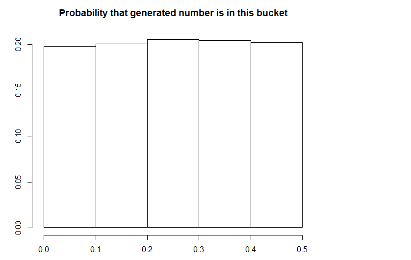
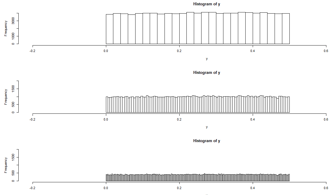
Let’s brute force our way through a problem of infinite possibilities. A simple example would be a random real number generator between 0 and 1/2. We generate 10000 numbers and bucket them into intervals of fixed width. E.g. We can see that roughly a fifth of the numbers would be between each 0.1 bucket But nothing stops us from fixing the bucket size, so we could make it smaller and smaller. As you can see, the heights get smaller and smaller since the probability of a number falling in a smaller bucket is small. And here is the heart of the problem. The PMF can never work for continuous distributions because it is guaranteed to give 0 probabilities for every bucket at infinite precision.
But continuous distributions don’t care about the resolution of a histogram. We both know our random-number-generator has a probability distribution. We just don’t know what it is. We need a better tool to map a continous distribution.

Part Three: The PDF (Probability Density Function)

Here’s the thing about continous distributions - there are infinite values in any bucket. Hence, a PMF with infinite resolution would give a decent approximation of the shape of the function even if it is at the cost of near-zero heights. So one could compromize on a decently large resolution and freeze the PMF so as to get the shape. Then the y-axis is rescaled such that the area under the shape becomes 1. In our case, this results in a rectangle with width 0.5 and height 2. This rescaling of y-axis itself is the normalizing factor, the per-ness in the density #bullshitspiration.

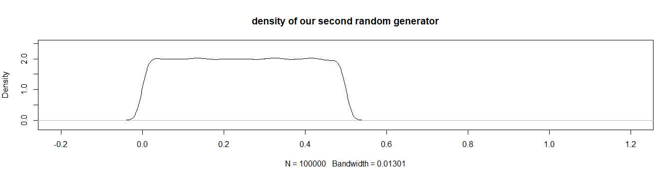
On a side note - Kernel Density Estimation - is all about finding the most accurate PDF from given observations/histogram/PMF. I used an r-based function called 'density' to arrive at the above graph which uses a very simple technique

Now how does one make sense of the graph? What does the 2 even mean?

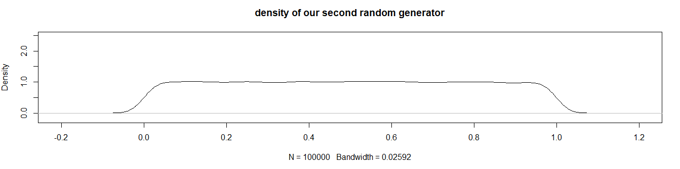
Let’s do a comparision with another simple number generator, this time the numbers are equally probable between 0 and 1. It’s PDF would look like as follows. The curve is much flatter, obviously, because the width of the rectangle is larger (remember the area has to be 1).
What does this say? The likelihood of generating a number around 0.2 (or any number between 0 and 0.5 because the PDFs are flat) is twice as much in our first distribution as compared to the second.

Let’s end with another example.

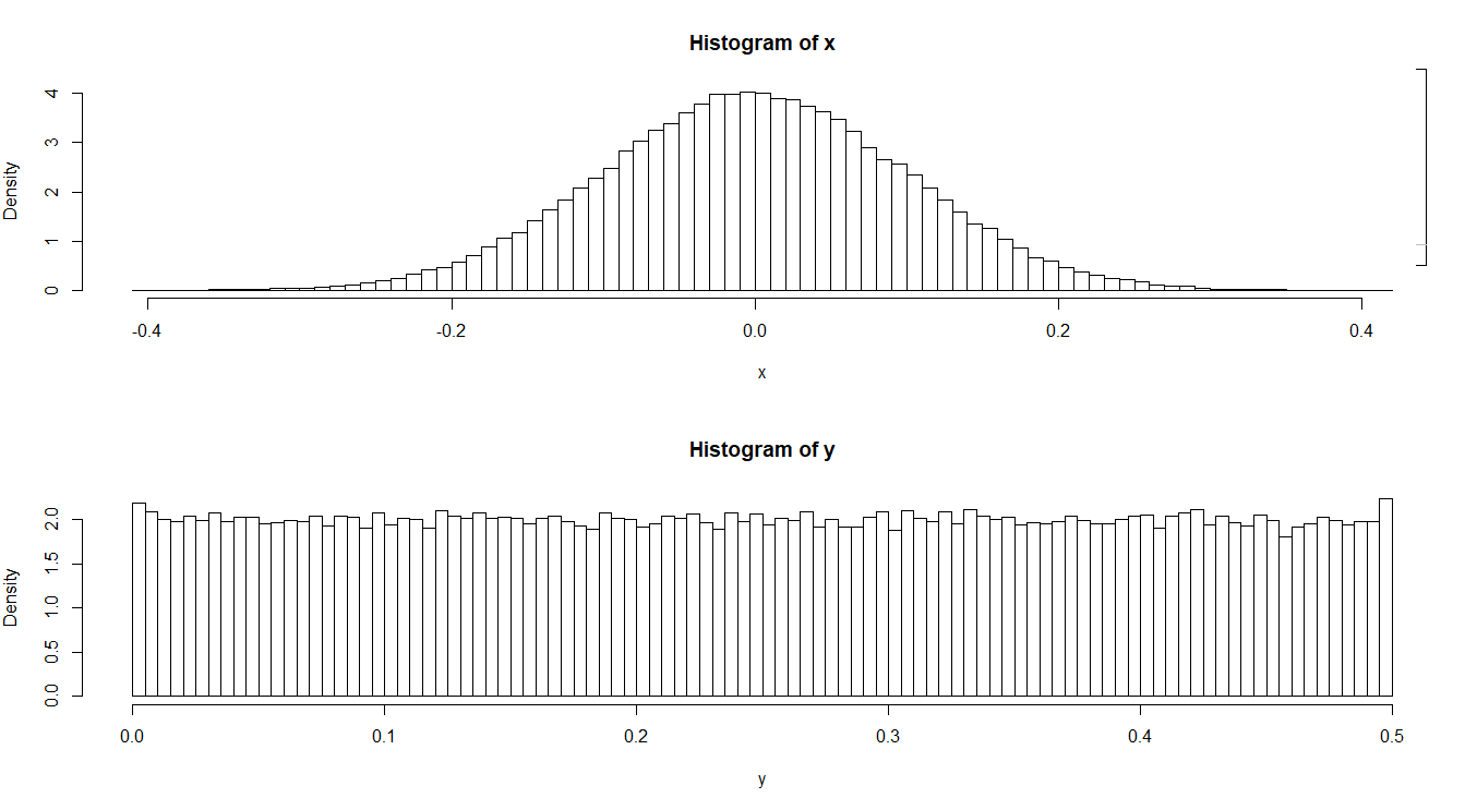
Given above are two probability distribution functions. We may know nothing about their statistics, but somethings we could say by simply looking -

1. The probability of getting/generating/finding a number around 0.0 in distribution ‘x’ is twice as much as getting a number around 0.0 in distribution ‘y’ (We are simply comparing the heights).
2. One is 4 times as likely to get a number around 0.0 than getting a number around 0.2 in the distribution ‘x’ (Now we are comparing outcomes from the same distribution. At 0.0 the height is ~4 and at at 0.2 it is ~1)
3. One is equally likely to get a number around 0.2 in ‘x’ and 0.3 in ‘y’ (The heights are pretty much the same)

So, there. Now you (I?) know that density by itself has no meaning. Now you know the philosophical meaning when Lao-Tzu says

So it is that existence and non-existence give birth the one to (the idea of) the other; that difficulty and ease produce the one (the idea of) the other; that length and shortness fashion out the one the figure of the other; that (the ideas of) height and lowness arise from the contrast of the one with the other; that the musical notes and tones become harmonious through the relation of one with another; and that being before and behind give the idea of one following another.